Tasked to complete weekly challenges covering concepts, principles, and algorithmic foundations
for robots and autonomous vehicles operating in the physical world for the class 6.141 (Robotics, Science, and Systems) at MIT.
Weekly challenges included designing and implementing wall following algorithms, visual servoing and lane following, localization, and
planning and trajectory following. The final challenge was to complete a lap of a race course with no collisions as fast as possible as well
as to navigate an obsticle course as fast as possible while minimizing collisions. Most of the class was done with the support of a team!
The first challenge was to individually implement a robust wall-following autonomous controller using a 2D racecar's LIDAR data. The racecar should drive
forward while maintaining a constant distance from the wall (either to the left or right of the car). We then worked in teams to implement this
on a 3D car simulator with realistic physics simulation. A combination of RANSAC, PID, and turn detection was used to implement the wall follower in 3D.
The RANSAC algorithm can take in the LIDAR data and determine the optimal fitting line that would represent the 'wall' (robust to outliers). The distance
between the car and wall can then be estimated using this drawn line and the error between the car's estimated distance from the wall and desired distance can be
fed into a PID controller to alter the car's steering. The LIDAR data can also be broken into different sections to identify upcoming turns and slow the car appropriately.
2. Visual Servoing
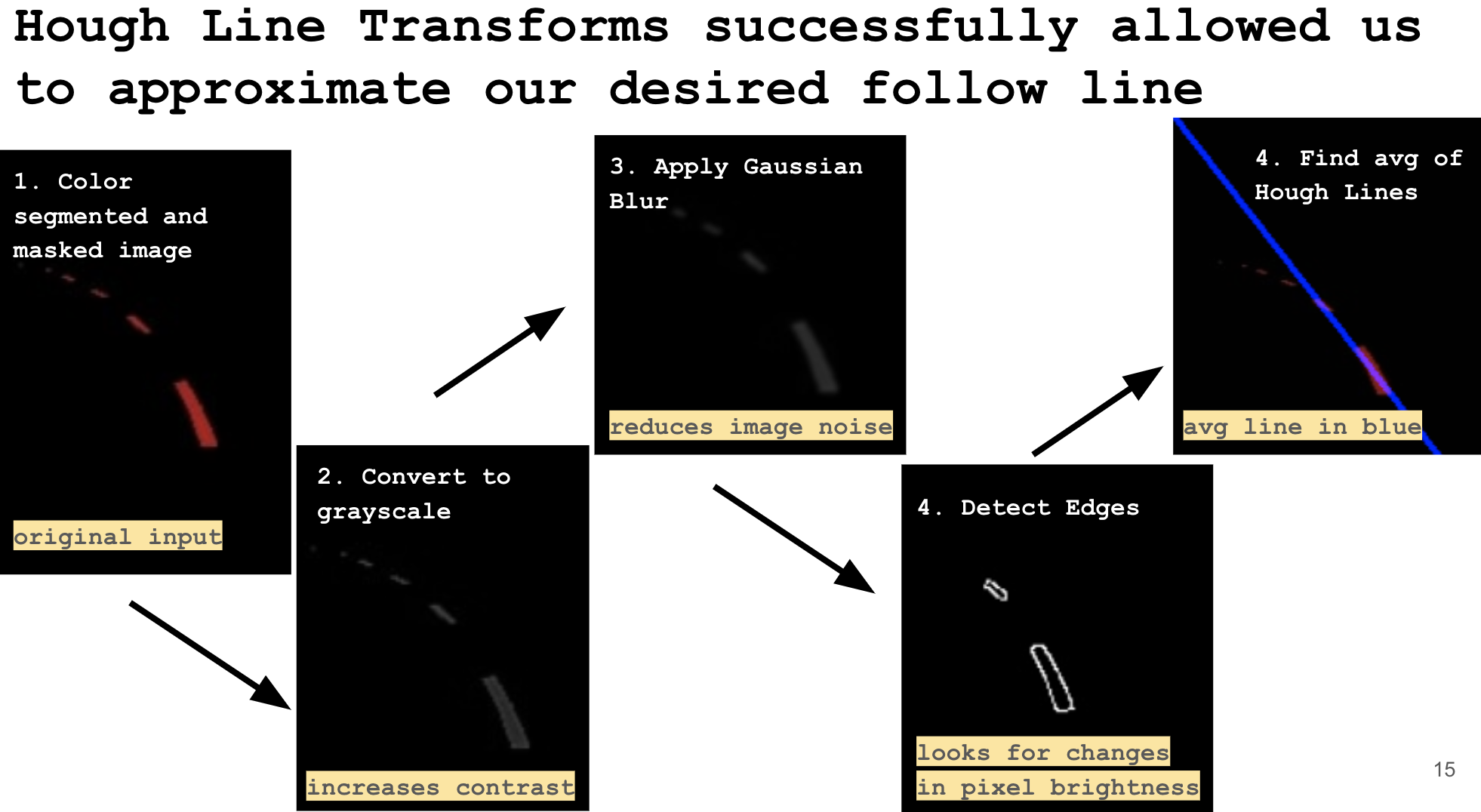
The second challenge was to implement a line follower and parking controller using computer vision. I spent most time
working on my team's line detection and following carrying some methods over from our wall follower and implementing
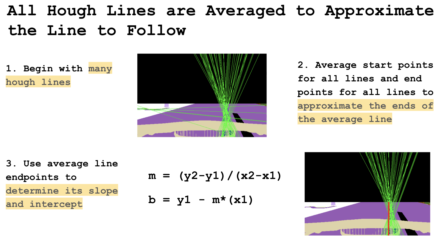
hough line transforms. Hough line transforms can be used to detect straight lines in an image. Averaging starting and
ending points for all detected hough lines can give an approximation for the average line and can be used as our line to
follow.
3. Localization
Localization is a key problem that must be solved when dealing with self-driving vehicles.
Localization allows the car/robot to know where it is physically within a known area or region.
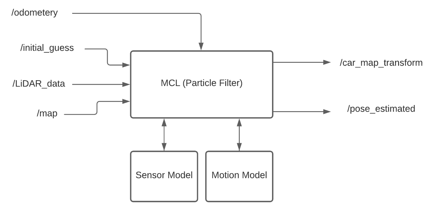
Our overall solution to this problem is shown below:
Monte Carlo Localization was used to solve the problem of localization.
A large number of particles represents possible positions of the robot. As the robot moves,
it's odometry information is used to propagate the particles accordingly (motion model). Then,
sensor (LIDAR) data is used to compute the probability of each particle being representative of the
robot's true location. I worked on implementing the vehicle's motion model. The
odometry data was calculated by integrating control and proprioceptive measure-
ments to estimate current pose given a known starting pose. More specifically,
this was done using the wheel odometry coming from dead-reckoning integration
of motor and steering commands. Because there are numerous factors that can
contribute to uncertainty in robot perception (wheel slip, gear backlash, mea-
surement noise, sensor or processor errors, and more), this uncertainty needs to
be included in our motion model. Random Gaussian noise was added to both
the odometry data as well as the particle poses directly to ensure that the particles will spread.
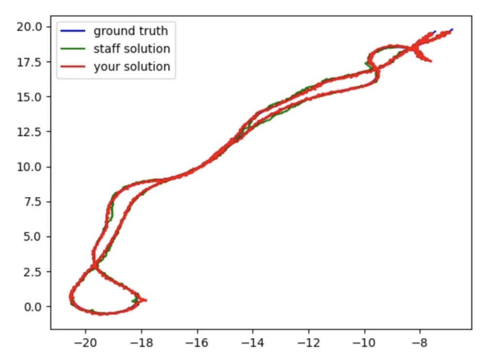
Below shows our localization implementation’s estimated pose as compared to
the ground truth pose and the TA solution with odometry noise.
4. Path Planning and Pure Pursuit
The goal for path planning was to quickly identify a trajectory (as direct as possible) between two points while
avoiding walls and obstacles. The Pure Pursuit controller for actually controling the movement of the car
needed to keep it on the planned path. I focused on the Pure Pursuit controller. To implement Pure Pursuit,
a reference point is first chosen on the desired trajectory a predefined
look ahead distance from the car. Then, a steering angle and velocity are
determined so that the car would hit the chosen reference point if the angle was kept constant. Below you
can see the results of our path planning and Pure Pursuit controller. The starting point for the
planned path for the final 2D implementation is shown in green while the end point is shown in red. The planned path is in white
and the orange point marks the location of the car as it followed the path under
Pure Pursuit control.
5. Final Challenge: Race and Obstacle Avoidance
Our final challenge was broken into two parts. The first was to finish a lap on a race track as quickly as possible with
no collisions. This was be done by designing the final race trajectory ourselves, using the TESSE car’s ground truth localization, and using
Pure Pursuit path following. The second part was fast obstacle avoidance. We had to reach the end of an obstructed road
while minimizing collisions and maximizing speed. This was done utilizing LIDAR to detect the obstacles,
path planning around the obstacles, and tracking collisions. I focused on the race track lap.
We successfully completed a lap around Windridge city in under about 49 seconds with no collisions.
Our solution was further optimized using path-segment-dependent variable look ahead distances
and velocities (for Pure Pursuit). On straightaways, the look ahead distance was much larger to minimize
oscillations and was decreased during turns. Our velocity controller increased
speed as the car started a segment, reaching a maximum in the middle of the segment, and reduced
velocity towards segment ends. Our final race track performance is shown below as well as write-ups for the
final challenge.